附录 L — 研究设计和数据构建
本文研究目的是呈现怎样通过微观个体「所得税-创新弹性」加总得到宏观「所得税创新-弹性」。因此,本部分依次介绍:模型设定、数据库构造、变量界定和统计描述。
L.1 变量和弹性的定义
创新活动需要发明人投入时间和原材料要素。个人所得税和公司所得税会通过影响发明人的投资回报率,进而影响其创新产出水平。
因此,就个人层面而言,个人所得税和公司所得税会影响发明人下述决策:
- 创新活动的工作时长和原材料投入;
- 职业选择 (选择受 雇佣于公司,还是 自雇佣);
- 迁移选择 (选择长居本州还是迁往其他州)。
作者构造了一个创新产出模型,以定量刻画微观个体发明人的不同决策行为。
L.1.1 A. 基本标记符号
假设发明人 \(i\) 在时期 \(t\) 居住在 \(s\) 州,
- 创新数量:\(y_{i s t}\)
- 创新质量:\(q_{i s t}\)
- 受雇于公司 (上标 \(^c\)):\(y_{i s t}^c\),\(q_{i s t}^c\)
- 自雇佣状态 (上标 \(^p\)):\(y_{i s t}^p\),\(q_{i s t}^p\)
- 创新产出来源于本州发明人 (上标 \(d\)): \(y_{i s t}^d\)
- 非本州:(上标 \(0\)): \(y_{i s t}^0\)
因此:
- 受雇于公司的发明人:\(I_{t}^{c} = I_{t}^{d, c} \cup I_{t}^{o, c}\)
- \(I_{t}^{d, c}\) 和 \(I_{t}^{o, c}\) 分别为在时期 \(t\) 定居于 \(s\) 州的发明人子集合和外来发明人子集合。
- 同理 (自雇),\(I_{t}^{p} = I_{t}^{d, p} \cup I_{t}^{o, p}\)
L.1.2 B. 创新产出-税收 关系
对于微观个体发明人,个人所得税、公司所得税与创新产出之间关系为:
\[ y_{i s t} = y_{i}\left(1-\tau_{s t}^{c},\ 1-\tau_{s t}^{p}\right) \]
\[ q_{i s t} = q_{i}\left(1-\tau_{s t}^{c},\ 1-\tau_{s t}^{p}\right) \]
L.1.3 C. 所得税-创新弹性
\(Y\):所得税-创新数量弹性
根据微观个体发明人的行为决策,首先,作者使用发明人的职业选择定义了四种 所得税-创新数量弹性:\(\{c,p\} \times \{\tau^{c},\tau^{p}\}\)。这里列出其中的四种:
- \(\varepsilon_{Y,p}^{c}\):受雇于公司的 发明人 个人 所得税净税率-创新数量弹性
- \(\varepsilon_{Y,c}^{c}\):受雇于公司的 发明人 公司 所得税净税率-创新数量弹性
- \(\varepsilon_{Y,p}^{p}\):自雇佣 发明人 个人 所得税净税率-创新数量弹性
- \(\varepsilon_{Y,c}^{p}\):自雇佣 发明人 公司 所得税净税率-创新数量弹性
\[ \varepsilon_{Y,\ p}^{c}:=\frac{\mathrm{d} log\left(y_{i s t}\right)}{\mathrm{d} log \left(1-\tau_{s t}^{p} \right)} \quad \varepsilon_{Y,\ c}^{c}:=\frac{\mathrm{d} log\left(y_{i s t}\right)}{\mathrm{d} log \left(1-\tau_{s t}^{c} \right)} \]
\[ \varepsilon_{Y,\ p}^{p}:=\frac{\mathrm{d} log\left(y_{i s t}\right)}{\mathrm{d} log(1-\tau_{s t}^{p})} \quad \varepsilon_{Y,\ p}^{c}:=\frac{\mathrm{d} log\left(y_{i s t}\right)}{\mathrm{d} log(1-\tau_{s t}^{c})} \]
Note: 「\(:=\)」符号的的含义是「定义为……」
\(Q\):所得税-创新质量弹性
只需把上式中的 \(Y\) 换成 \(Q\) 即可:\(\varepsilon_{Q,\ p}^{c}\)、\(\varepsilon_{Q,\ c}^{c}\)、\(\varepsilon_{Q,\ p}^{p}\)、\(\varepsilon_{Q,\ c}^{p}\)
\(d-o\):所得税-迁移弹性
作者根据发明人的迁移决策定义了四类 所得税-迁移弹性,即本州居民的个人所得税净税率-迁移弹性 (\(\eta_{p}^{d}\))、本州居民的公司所得税净税率-迁移弹性 (\(\eta_{c}^{d}\))、外来居民的个人所得税净税率-迁移弹性 (\(\eta_{p}^{o}\)) 和外来居民的公司所得税净税率-迁移弹性 (\(\eta_{c}^{o}\)):
\[ \eta_{p}^{d} := \frac{\mathrm{d} log \left(\int_{i \in I^{d}} d i \right)}{\mathrm{d} log \left(1-\tau^{p}\right)} \quad \eta_{c}^{d} := \frac{\mathrm{d} log \left(\int_{i \in I^{d}} d i \right)}{\mathrm{d} log \left(1-\tau^{c}\right)} \]
\[ \eta_{p}^{o} := \frac{\mathrm{d} log \left(\int_{i \in I^{o}} o i \right)}{\mathrm{d} log \left(1-\tau^{p}\right)} \quad \eta_{c}^{o} := \frac{\mathrm{d} log \left(\int_{i \in I^{o}} o i \right)}{\mathrm{d} log \left(1-\tau^{c}\right)} \]
微观弹性与宏观弹性的关系
如果州层级的创新产出数量和质量满足:
- \(Y:=\int_{i \in I^{d} \cup I^{o}} y_{i} d i\) \(Q:=\int_{i \in I^{d} \cup I^{o}} y_{i} d i\)
则 州层级 的「所得税净税率-创新数量弹性」可以表示为:
\[ \varepsilon_{Y,\ p}:=\frac{d \log (Y)}{d \log \left(1-\tau^{p}\right)}=\gamma_{Y}^{c} \varepsilon_{Y,\ p}^{c}+\left(1-\gamma_{Y}^{c}\right) \varepsilon_{Y,\ p}^{p}+\gamma_{Y}^{d} \eta_{p}^{d}+\left(1-\gamma_{Y}^{d}\right) \eta_{p}^{o} \quad \text{(1)} \]
\[ \varepsilon_{Q, p}:=\frac{d \log (Q)}{d \log \left(1-\tau^{p}\right)}=\gamma_{Q}^{c} \varepsilon_{Q, p}^{c}+\left(1-\gamma_{Q}^{c}\right) \varepsilon_{Q, p}^{p}+\gamma_{Q}^{d} \eta_{p}^{d}+\left(1-\gamma_{Q}^{d}\right) \eta_{p}^{o} \quad \text{(2)} \]
其中,
- \(\gamma_{Y}^{c}\)、\(\gamma_{Y}^{d}\)、\(\gamma_{Q}^{c}\) 和 \(\gamma_{Q}^{d}\) 分别表示受雇佣于公司发明人创新数量占比、本州发明人创新数量占比、受雇于公司发明人创新质量占比、本州发明人创新质量占比。
- 作为互斥集合,自雇佣发明人创新数量占比、外来发明人创新数量占比、自雇佣发明人专利质量占比、外来发明人创新质量占比分别为 \(\left(1-\gamma_{Y}^{c}\right)\)、\(\left(1-\gamma_{Y}^{d}\right)\)、\(\left(1-\gamma_{Q}^{c}\right)\) 和 \(\left(1-\gamma_{Q}^{d}\right)\)。
公式 (1) 和公式 (2) 将用于第五部分计算微观个体发明人创新产出弹性的加总值。
L.2 数据构建
作者构建了四个历史数据集:
- 发明人历史面板数据库,这些数据来源于数字专利数据库 (1920-2000 年)。这个数据库能够追踪每一个发明人的专利数量、专利引用数量、居住地、技术领域和是否转让专利权给公司。
- 州层级的历史公司所得税数据库。
- 使用 Bakijia (2006) (Note:只找到了 2009 的版本) 方法构建了一个个人所得税数据库。
- 合并上述数据库后,进一步增加了一些额外的与创新相关的衡量指标,如专利的市场价值 (Kogan et al.,2017) 和州层级的价值增加值、制造业的 GDP 占比、平均周薪、机构数量、总薪酬支出 (Allen, 2004; Haines, 2010)。
上述数据库的具体调整过程,查看 附录。
Table Ⅰ是文中涉及到的主要变量的描述性统计结果,其具体作用下文详述。
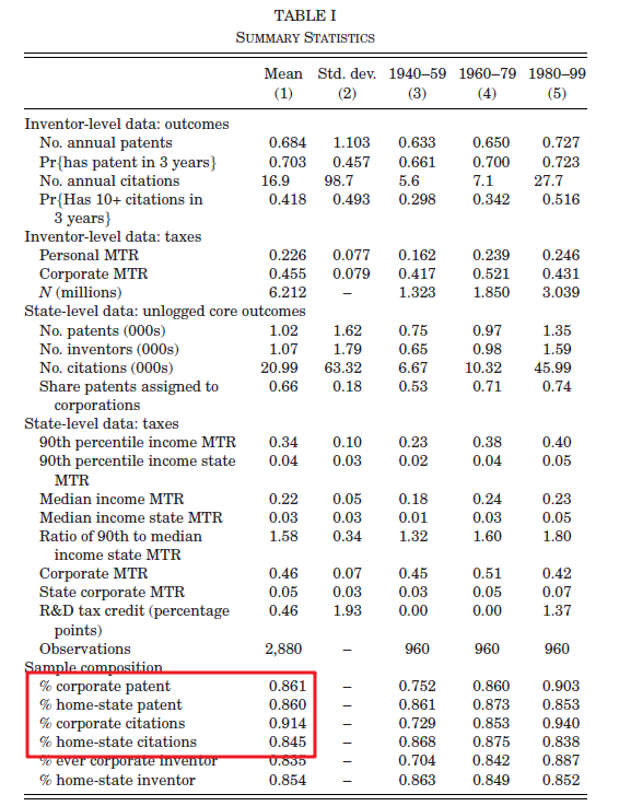
Notes. This table reports summary statistics for our estimation sample. This includes all mainland U.S. states, excluding Louisiana, from 1940 to 2000 . Columns (1) and (2) report the mean and standard deviation, respectively, for the full sample period, and columns (3)-(5) report the averages in each 20 -year period from 1940 to 2000. “State MTR” refers to the state’s marginal tax rate excluding federal taxes, and “MTR” refers to tax rates inclusive of federal and state tax liabilities. “Home-state patents” are patents granted to inventors who live in the state in which they first appear in the data. Additional summary statistics, including those regarding logged outcome variables, corporate tax base rules, other outcome variables, and control variables are included in Online Appendix Table C.2. Inventors are included between the years of their first successful patent application and their last successful patent application. Inventor-level summary statistics are averaged over inventor-year observations to reflect summary statistics of our estimation sample. More summary statistics are in Online Appendix C.
L.3 MTR:税率指标
- the 90 th percentile income MTR, (denoted by MTR90 for conciseness).
- the 90 th percentile income ATR, (denoted by ATR90)
- the median income MTR, (denoted by MTR50)
- the median income ATR, (denoted by ATR50).
L.4 个税变化时序特征
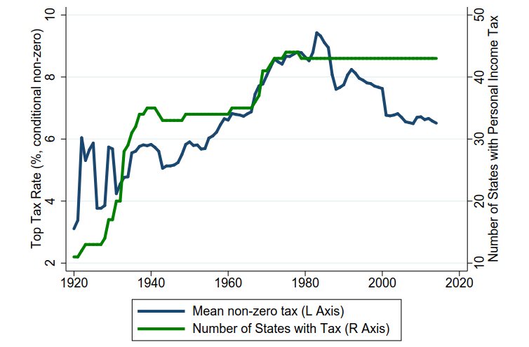
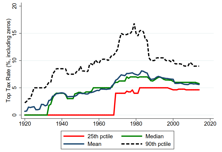
Figure C.5: Figure plots the share of states with a personal income tax, as well as the distribution of those taxes over time.
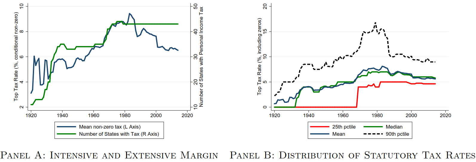
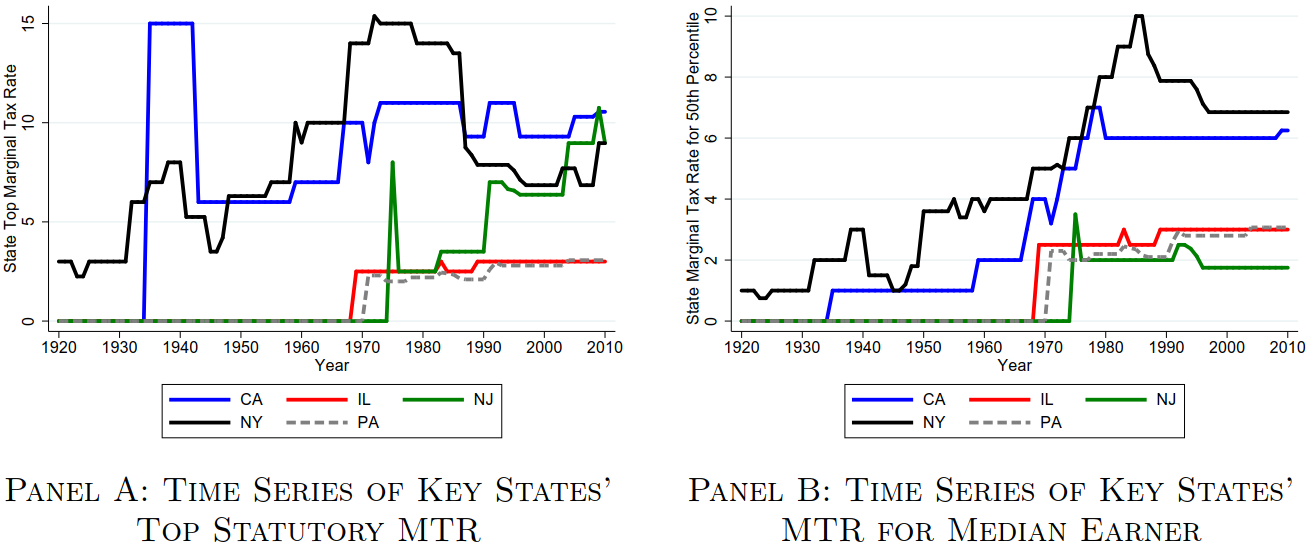
Figure C.8: Figure plots the time series of marginal personal income tax rates for the five most innovative states in our sample. Tax rates are measured in percentage points. Panel A shows the top statutory personal income tax rate, while Panel B plots it for the median earner. 州名缩写 - CA-加州;IL-伊利诺斯;NJ-新泽西;NY-纽约州;PA-宾夕法尼亚州