# -*- coding: utf-8 -*-
"""
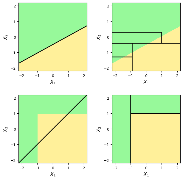
绘制线性分类器与决策树分类边界的对比图。
"""

import os
import numpy as np
import matplotlib.pyplot as plt
from matplotlib.colors import ListedColormap

# ── 1. 基本设置 ─────────────────────────────────────────────
os.makedirs("./figs", exist_ok=True)

# 图形颜色:0 表示黄色区域,1 表示绿色区域
YELLOW = "#FFF09A"
GREEN = "#97F99A"
CMAP = ListedColormap([YELLOW, GREEN])

# 坐标范围
x_min, x_max = -2.2, 2.2
y_min, y_max = -2.2, 2.2

# 用网格点生成二维平面
x1 = np.linspace(x_min, x_max, 500)
x2 = np.linspace(y_min, y_max, 500)
X1, X2 = np.meshgrid(x1, x2)

# ── 2. 构造真实的分类区域 ──────────────────────────────────
Z_linear = (X2 >= 0.55 * X1 - 0.50).astype(int)
Z_nonlinear = np.where((X1 >= -1.0) & (X2 <= 1.0), 0, 1)

# ── 3. 辅助函数 ────────────────────────────────────────────
def format_axis(ax):
    """统一设置坐标轴格式。"""
    ax.set_xlim(x_min, x_max)
    ax.set_ylim(y_min, y_max)
    ax.set_aspect("equal", adjustable="box")
    ax.set_xlabel(r"$X_1$", fontsize=11)
    ax.set_ylabel(r"$X_2$", fontsize=11)
    ax.set_xticks([-2, -1, 0, 1, 2])
    ax.set_yticks([-2, -1, 0, 1, 2])
    ax.tick_params(axis="both", labelsize=9, direction="out")
    for spine in ax.spines.values():
        spine.set_linewidth(0.8)

def draw_region(ax, Z):
    """绘制分类区域。"""
    ax.contourf(X1, X2, Z, levels=[-0.5, 0.5, 1.5], cmap=CMAP, alpha=1.0)

# ── 4. 绘制图形 ────────────────────────────────────────────
fig, axes = plt.subplots(2, 2, figsize=(7.2, 7.0))

xx = np.linspace(x_min, x_max, 200)

# 左上:线性边界 + 线性模型
axes[0, 0].contourf(X1, X2, Z_linear, levels=[-0.5, 0.5, 1.5], cmap=CMAP, alpha=1.0)
axes[0, 0].plot(xx, 0.55 * xx - 0.50, color="black", linewidth=1.8)
format_axis(axes[0, 0])

# 右上:线性边界 + 决策树模型
axes[0, 1].contourf(X1, X2, Z_linear, levels=[-0.5, 0.5, 1.5], cmap=CMAP, alpha=1.0)
axes[0, 1].hlines(y=-0.40, xmin=x_min, xmax=x_max, color="black", linewidth=1.8)
axes[0, 1].vlines(x=-0.90, ymin=y_min, ymax=-0.40, color="black", linewidth=1.8)
axes[0, 1].hlines(y=-1.30, xmin=x_min, xmax=-0.90, color="black", linewidth=1.8)
axes[0, 1].hlines(y=0.30, xmin=x_min, xmax=1.00, color="black", linewidth=1.8)
axes[0, 1].vlines(x=1.00, ymin=-0.40, ymax=0.30, color="black", linewidth=1.8)
format_axis(axes[0, 1])

# 左下:非线性边界 + 线性模型
axes[1, 0].contourf(X1, X2, Z_nonlinear, levels=[-0.5, 0.5, 1.5], cmap=CMAP, alpha=1.0)
axes[1, 0].plot(xx, xx, color="black", linewidth=1.8)
format_axis(axes[1, 0])

# 右下:非线性边界 + 决策树模型
axes[1, 1].contourf(X1, X2, Z_nonlinear, levels=[-0.5, 0.5, 1.5], cmap=CMAP, alpha=1.0)
axes[1, 1].vlines(x=-1.00, ymin=y_min, ymax=y_max, color="black", linewidth=1.8)
axes[1, 1].hlines(y=1.00, xmin=-1.00, xmax=x_max, color="black", linewidth=1.8)
format_axis(axes[1, 1])

plt.subplots_adjust(wspace=0.28, hspace=0.35)
fig.savefig("./figs/ml_tree_fig02_linear_tree_boundary.png", dpi=300, bbox_inches="tight")
fig.savefig("./figs/ml_tree_fig02_linear_tree_boundary.svg", bbox_inches="tight")
plt.show()