课程 :部分线性函数型面板数据模型 (PLFC)
数据来源 :Du et al. (2021), Energy Economics
目标 :理解样条基函数如何逼近未知的函数系数 γ(U)
数据准备
使用 Du et al. (2021) 的中国城市面板数据。
use "https://github.com/lianxhcn/data/raw/refs/heads/main/stata/Du2021EE_ERdata.dta" , clear year
(Du et al. (2021, EE) https://doi.org/10.1016/j.eneco.2021.105247)

Panel variable: cityno (strongly balanced)
 Time variable: year, 2002 to 2015
         Delta: 1 unit
describe gti er gdp rd pop hc inv fdi
Variable      Storage   Display    Value
    name         type    format    label      Variable label
-------------------------------------------------------------------------------
gti             int     %10.0g                Green technology patents
                                                (authorized, by application
                                                date)
er              double  %10.0g                ER: environmental regulation
                                                index (entropy-weight
                                                composite)
gdp             double  %10.0g                Real GDP per capita (2001
                                                constant prices)
rd              double  %10.0g                Fiscal exp. on tech & education /
                                                GDP
pop             double  %10.0g                Population (10,000 persons)
hc              double  %10.0g                High school students (1,000
                                                persons)
inv             double  %10.0g                Fixed-asset investment / GDP
fdi             double  %10.0g                FDI / GDP
tabstat lngti er lngdp lnrd lnpop lnhc lninv lnfdi, /// s (n mean sd min max ) c(s )
    Variable |         N      Mean        SD       Min       Max
-------------+--------------------------------------------------
       lngti |   1470.00      4.32      1.89      0.00      9.53
          er |   1470.00      0.08      0.04      0.02      0.45
       lngdp |   1470.00     10.09      0.67      8.12     11.76
        lnrd |   1470.00     -0.06      0.61     -1.84      1.65
       lnpop |   1470.00      6.11      0.72      3.31      8.01
        lnhc |   1470.00      4.29      1.36     -0.27      6.95
       lninv |   1470.00      3.95      0.42      2.46      5.10
       lnfdi |   1470.00      0.47      1.19     -6.01      3.00
----------------------------------------------------------------
变量说明 :
lngti: 绿色技术创新(对数)er: 环境规制强度lngdp: 人均 GDP(对数)—— 调节变量 Ulnrd: 科技与教育经费投入lnpop: 城市规模lnhc: 人力资本lninv: 固定资产投资lnfdi: 经济开放度
手动构造样条基函数
为了深入理解 xtplfc 的工作原理,我们先手动构造三次样条基函数。
Step 1: 确定样条结点位置
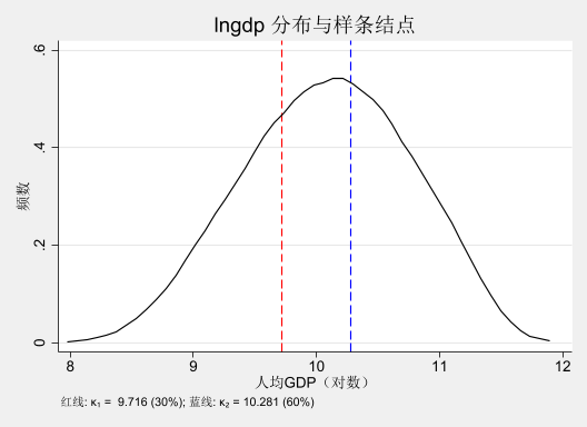
选择 lngdp 的 30% 和 60% 分位点作为结点。
use "https://github.com/lianxhcn/data/raw/refs/heads/main/stata/Du2021EE_ERdata.dta" , clear p (30 60)global knot1: dis %6.3f r (r1) global knot2: dis %6.3f r (r2) display "Knot 1 (30th percentile): " $knot1 display "Knot 2 (60th percentile): " $knot2
Running D:\stata19/profile.do ...
(Du et al. (2021, EE) https://doi.org/10.1016/j.eneco.2021.105247)
Knot 1 (30th percentile): 9.716
Knot 2 (60th percentile): 10.281
kdensity lngdp, /// xline ($knot1 , lcolor(red ) lpattern(dash )) /// xline ($knot2 , lcolor(blue ) lpattern(dash )) /// xtitle ("人均GDP(对数)" ) /// ytitle ("频数" ) /// title ("lngdp 分布与样条结点" ) /// note ("红线: κ₁ = $knot1 (30%); 蓝线: κ₂ = $knot2 (60%)" ) /// scheme (s2mono)
2.2 Step 2: 构造三次样条基函数
构造 6 个基函数: - h1 = 1 (常数项) - h2 = U (线性项) - h3 = U² (二次项) - h4 = U³ (三次项) - h5 = (U - κ₁)³₊ (第一个样条调整项) - h6 = (U - κ₂)³₊ (第二个样条调整项)
gen h1 = 1 // Stata 会自动加入常数项,因此不需要这一项 gen h2 = lngdpgen h3 = lngdp^2gen h4 = lngdp^3gen h5 = (lngdp - $knot1 )^3 if lngdp > $knot1 replace h5 = 0 if lngdp <= $knot1 gen h6 = (lngdp - $knot2 )^3 if lngdp > $knot2 replace h6 = 0 if lngdp <= $knot2
(441 missing values generated)
(441 real changes made)
(884 missing values generated)
(884 real changes made)
summarize h2-h6
    Variable |        Obs        Mean    Std. dev.       Min        Max
-------------+---------------------------------------------------------
          h2 |      1,470    10.08827    .6711921   8.116106   11.75655
          h3 |      1,470    102.2234    13.49979   65.87118   138.2164
          h4 |      1,470    1040.305    204.7095   534.6175   1624.947
          h5 |      1,470    .5914555    1.111614          0   8.496483
          h6 |      1,470    .1070663     .308674          0   3.212612
Step 3: 构造交互项 (Z × h)
将环境规制(er)与每个基函数相乘,得到 6 个交互项。
核心思想 :原模型 \(Y=\gamma(U) Z+\beta X+\alpha\) ,其中 \(\gamma(U) \approx \sum \theta_j {\color{blue}{h_j(U)}}\)
因此,
\[Y \approx \sum \theta_j\left[Z \cdot {\color{blue}{h_j(U)}}\right]+\beta X+\alpha\]
即 \(Z \cdot {\color{blue}{h_j(U)}}\) 成为新的解释变量。
forvalues j = 2/6 {gen h`j' _er = h`j' * erds h *_er
h2_er h3_er h4_er h5_er h6_er
估计模型(手动方法)
使用 reghdfe 吸收城市固定效应,等价于先一阶差分再 OLS。
ssc install reghdfe, replace
/// /// vce (cluster cityno)est store manual_est // 存结果
(MWFE estimator converged in 1 iterations)

HDFE Linear regression                            Number of obs   =      1,470
Absorbing 1 HDFE group                            F(  10,    104) =     138.27
Statistics robust to heteroskedasticity           Prob > F        =     0.0000
                                                  R-squared       =     0.9354
                                                  Adj R-squared   =     0.9299
                                                  Within R-sq.    =     0.8211
Number of clusters (cityno)  =        105         Root MSE        =     0.4998

                               (Std. err. adjusted for 105 clusters in cityno)
------------------------------------------------------------------------------
             |               Robust
       lngti | Coefficient  std. err.      t    P>|t|     [95% conf. interval]
-------------+----------------------------------------------------------------
       h2_er |   -111.508     35.145    -3.17   0.002     -181.201     -41.814
       h3_er |     21.648      7.176     3.02   0.003        7.417      35.878
       h4_er |     -1.050      0.367    -2.86   0.005       -1.777      -0.323
       h5_er |      7.731      4.230     1.83   0.071       -0.658      16.120
       h6_er |     -9.640      6.283    -1.53   0.128      -22.099       2.819
        lnrd |      0.785      0.129     6.10   0.000        0.530       1.041
       lnpop |      2.231      0.390     5.72   0.000        1.458       3.004
        lnhc |      0.453      0.150     3.02   0.003        0.155       0.751
       lninv |      0.461      0.156     2.95   0.004        0.151       0.771
       lnfdi |     -0.052      0.034    -1.54   0.126       -0.119       0.015
       _cons |    -13.037      2.120    -6.15   0.000      -17.241      -8.832
------------------------------------------------------------------------------

Absorbed degrees of freedom:
-----------------------------------------------------+
 Absorbed FE | Categories  - Redundant  = Num. Coefs |
-------------+---------------------------------------|
      cityno |       105         105           0    *|
-----------------------------------------------------+
* = FE nested within cluster; treated as redundant for DoF computation
结果解读 :
h2_er 到 h6_er 的系数即为 \(\theta_2\) 到 \(\theta_6\) 这些系数本身不直接解释,需要组合成 \(\gamma(U)\)
计算边际效应 γ(U)
由于模型中包含了拐点项,即 \((U - \kappa_k)^3_+\) ,我们无法使用 margins 命令计算边际效应。此时,需要借助 predictnl 命令来计算每个观测点的边际效应,即
\[\hat{\gamma}(U_i) = \sum_{j=2}^{6} \hat{\theta}_j h_j(U_i)\]
标准误可以使用 predictnl 的 se() 选项计算,详情参见 [R] predictnl
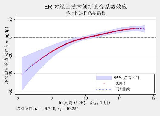
drop gamma_hat drop gamma_sepredictnl gamma_hat = _b[h2_er] * lngdp /// /// /// max (lngdp - $knot1 , 0)^3 /// max (lngdp - $knot2 , 0)^3, /// gen gamma_lb = gamma_hat - 1.96 * gamma_segen gamma_ub = gamma_hat + 1.96 * gamma_selabel var gamma_hat "ER 对 GTI 的边际效应" label var gamma_lb "95% CI 下界" label var gamma_ub "95% CI 上界"
summarize gamma_hat gamma_se gamma_lb gamma_ub
    Variable |        Obs        Mean    Std. dev.       Min        Max
-------------+---------------------------------------------------------
   gamma_hat |      1,470   -.9434624     7.80896  -40.47254   9.881587
    gamma_se |      1,470    1.705248    .9714625   1.120716   9.403664
    gamma_lb |      1,470   -4.285748    9.511348  -58.90372   6.931313
    gamma_ub |      1,470    2.398824    6.224541  -22.04136    13.4857
结果可视化
基本散点图 + 置信区间
twoway (rarea gamma_lb gamma_ub lngdp, color (blue *0.2) sort ) /// scatter gamma_hat lngdp, msize(tiny) mcolor(red %30)) /// blue %60) lwidth(thick) degree(3)), /// yline (0, lcolor(gray ) lp(dash )) /// xtitle ("ln(人均 GDP),滞后 1 期)" , size (medium)) /// ytitle ("环境规制的边际效应 γ(lngdp)" , size (medium)) /// title ("ER 对绿色技术创新的变系数效应" , size (large)) /// subtitle ("手动构造样条基函数" , size (medium)) /// legend (order (1 "95% 置信区间" 2 "预测值" 3 "平滑曲线" ) /// ring (0) pos(5) cols (1)) /// note ("结点位置: κ₁ = $knot1, κ₂ = $knot2" , size (*1.3)) /// scheme (s2mono)
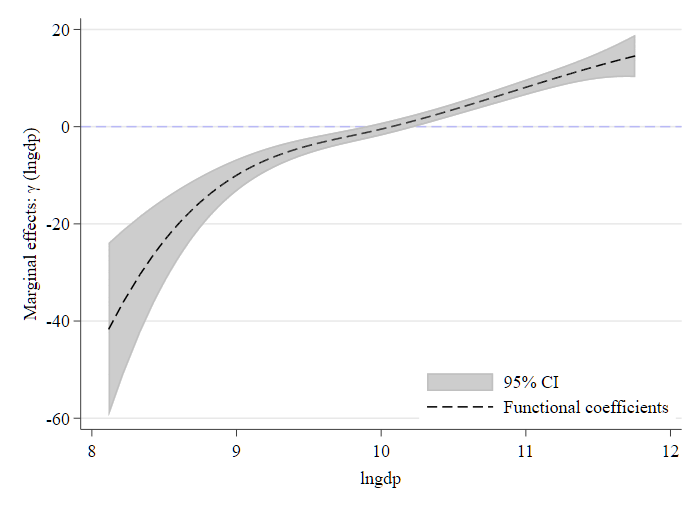
原文 结果:
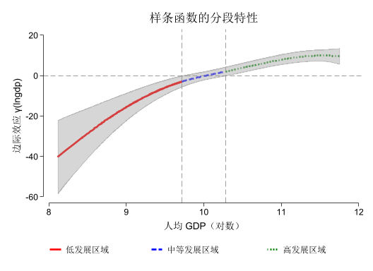
分段绘制(展示样条的分段特性)
preserve collapse (mean ) gamma_hat gamma_lb gamma_ub, by (lngdp)gen region = 1 if lngdp <= $knot1 replace region = 2 if lngdp > $knot1 & lngdp <= $knot2 replace region = 3 if lngdp > $knot2 label define region_lab 1 "低发展水平" 2 "中等发展水平" 3 "高发展水平" label values region region_labtwoway (line gamma_hat lngdp if region==1, lw(*2.5) lc(red ) ) /// line gamma_hat lngdp if region==2, lw(*2.5) lc(blue )) /// line gamma_hat lngdp if region==3, lw(*2.5) lc(green ) ) /// color (black *0.5%40)), /// yline (0, lc(black *0.6) lp(dash ) lw(*0.6)) /// xline ($knot1 $knot2 , lcolor(black *0.6) lp(dash ) lw(*0.6)) /// xtitle ("人均 GDP(对数)" ) /// ytitle ("边际效应 γ(lngdp)" ) /// title ("样条函数的分段特性" ) /// legend (order (1 "低发展区域" 2 "中等发展区域" 3 "高发展区域" ) /// r (1) ) /// scheme (scientific)restore
(Note: Below code run with echo to enable preserve/restore functionality.)


(1,016 missing values generated)

(438 real changes made)

(578 real changes made)
使用 xtplfc 命令
现在我们使用 xtplfc 命令重新估计,并与手动结果对比。
all replace from(http://www.stata-journal.com/software/sj20-4)
模型设定
由前文介绍可知,函数系数模型的一般形式为:
\[Y = \gamma(U) Z + \beta X + \alpha + \epsilon\]
我们关心的是 \(Z\) 对 \(Y\) 的边际影响 \(\gamma(U)\) ,尤其是 \(\gamma(U)\) 随调节变量 \(U\) 的变化情况。
Du et al. (2021) 中的模型设定为:
\[lngti_{it} = \gamma(lngdp_{it-1}) er_{it} + \beta X_{it} + \alpha_i + \epsilon_{it}\]
对应关系为:\(Y = lngti_{it}\) ,\(U = lngdp_{it-1}\) ,\(Z = er_{it}\)
drop fcoe_gti* local controls "lnrd lnpop lnhc lninv lnfdi" `controls' , /// /// /// gen (fcoe_gti) /// quantile ///
Computing the bootstrap standard errors...
.................................................50
.................................................100
.................................................150
.................................................200

Partially linear functional-coefficient panel data model.
Fixed-effect series semiparametric estimation.
Estimation results: linear part                 Number of obs        =    1365
                                                Within R-squared     =  0.1754
                                                Adj Within R-squared =  0.1693
                                                Root MSE             =  0.4291
------------------------------------------------------------------------------
       lngti | Coefficient  Std. err.      z    P>|z|     [95% conf. interval]
-------------+----------------------------------------------------------------
        lnrd |      0.089      0.048     1.84   0.066       -0.006       0.184
       lnpop |      1.637      0.232     7.06   0.000        1.183       2.091
        lnhc |      0.216      0.076     2.86   0.004        0.068       0.364
       lninv |      0.392      0.078     5.00   0.000        0.238       0.546
       lnfdi |      0.015      0.018     0.81   0.419       -0.021       0.050
------------------------------------------------------------------------------
Estimated functional coefficient(s) are saved in the data.
注 :上述命令中的关键选项说明如下:
gen(fcoe_gti):指定变量名前缀,用于存储 及其标准误。程序会自动生成以下变量:
fcoe_gti_1:\(\gamma(U)\) 的估计值 \(\hat{\gamma}(U)\) fcoe_gti_1_sd:\(\gamma(U)\) 的标准误 \(se(\hat{\gamma}(U))\) (通过 Bootstrap 得到) brep(200):指定 Bootstrap 重抽样次数为 200 次,以估计 \(\hat{\gamma}(U)\) 的标准误 (后面绘图时会用到)。
本例中为了节省运行时间,将抽样次数设为 200,实际应用时建议设为 1000 次或更多。
gen fcoe_lb = fcoe_gti_1 - 1.96 * fcoe_gti_1_sdgen fcoe_ub = fcoe_gti_1 + 1.96 * fcoe_gti_1_sd
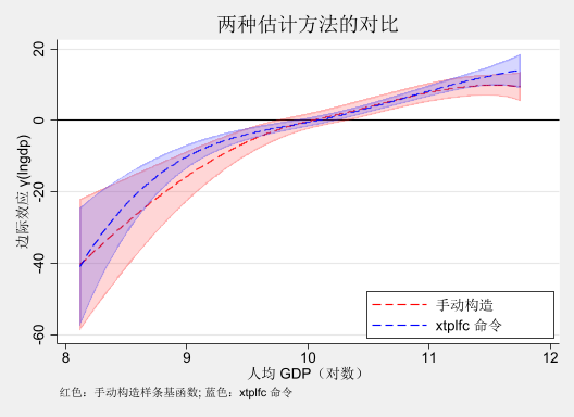
对比两种方法的结果
(obs=1,470)

             | gamma_~t fcoe_g~1
-------------+------------------
   gamma_hat |   1.0000
  fcoe_gti_1 |   0.9843   1.0000
twoway (rarea gamma_lb gamma_ub lngdp, color (red %20) sort ) /// line gamma_hat lngdp, lcolor(red ) lwidth(medium) sort ) /// color (blue %20) sort ) /// line fcoe_gti_1 lngdp, lcolor(blue ) lwidth(medium) lpattern(dash ) sort ), /// yline (0, lcolor(black )) /// xtitle ("人均 GDP(对数)" ) /// ytitle ("边际效应 γ(lngdp)" ) /// title ("两种估计方法的对比" ) /// legend (order (2 "手动构造" 4 "xtplfc 命令" ) /// ring (0) pos(5) c(1)) /// note ("红色:手动构造样条基函数; 蓝色:xtplfc 命令" ) /// scheme (s2mono)
稳健性检验
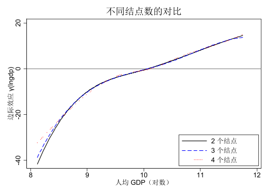
有些读者可能会担心,样条基函数的选择(如结点位置、次数等)会不会对结果产生较大影响。为此,我们可以尝试不同的结点位置和次数,观察估计结果的稳定性。
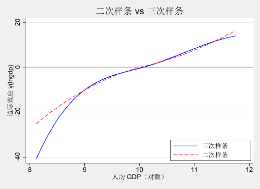
对比结果显示,无论是改变节点数 (使用 3 个节点和 4 个节点),还是改变次数 (使用二次和三次样条),得到的结果与上文基本设定下的结果都不存在显著差异。这说明,估计结果对样条基函数的选择较为稳健。这也是样条方法的一个重要优点。
改变结点数量
drop fcoe_3knots*/// /// gen (fcoe_3knots) /// quantile brep(10)
Computing the bootstrap standard errors...
..........
Partially linear functional-coefficient panel data model.
Fixed-effect series semiparametric estimation.
Estimation results: linear part                 Number of obs        =    1365
                                                Within R-squared     =  0.1749
                                                Adj Within R-squared =  0.1682
                                                Root MSE             =  0.4294
------------------------------------------------------------------------------
       lngti | Coefficient  Std. err.      z    P>|z|     [95% conf. interval]
-------------+----------------------------------------------------------------
        lnrd |      0.088      0.025     3.51   0.000        0.039       0.138
       lnpop |      1.630      0.271     6.01   0.000        1.098       2.163
        lnhc |      0.217      0.080     2.73   0.006        0.061       0.373
       lninv |      0.396      0.102     3.89   0.000        0.196       0.595
       lnfdi |      0.015      0.018     0.80   0.426       -0.021       0.050
------------------------------------------------------------------------------
Estimated functional coefficient(s) are saved in the data.
drop fcoe_4knots*/// /// gen (fcoe_4knots) /// quantile brep(100)
Computing the bootstrap standard errors...
.................................................50
.................................................100

Partially linear functional-coefficient panel data model.
Fixed-effect series semiparametric estimation.
Estimation results: linear part                 Number of obs        =    1365
                                                Within R-squared     =  0.1771
                                                Adj Within R-squared =  0.1698
                                                Root MSE             =  0.4289
------------------------------------------------------------------------------
       lngti | Coefficient  Std. err.      z    P>|z|     [95% conf. interval]
-------------+----------------------------------------------------------------
        lnrd |      0.090      0.047     1.93   0.054       -0.001       0.182
       lnpop |      1.670      0.267     6.26   0.000        1.147       2.193
        lnhc |      0.210      0.081     2.60   0.009        0.052       0.369
       lninv |      0.388      0.077     5.06   0.000        0.238       0.539
       lnfdi |      0.015      0.018     0.84   0.398       -0.020       0.050
------------------------------------------------------------------------------
Estimated functional coefficient(s) are saved in the data.
twoway (line fcoe_gti_1 lngdp, lc(black ) lwidth(medium) sort ) /// line fcoe_3knots_1 lngdp, lc(blue ) lpattern(dash ) sort ) /// line fcoe_4knots_1 lngdp, lc(red ) lpattern(dot ) sort ), /// yline (0, lcolor(gray )) /// xtitle ("人均 GDP(对数)" ) /// ytitle ("边际效应 γ(lngdp)" ) /// title ("不同结点数的对比" ) /// legend (order (1 "2 个结点" 2 "3 个结点" 3 "4 个结点" ) /// ring (0) pos(5) c(1)) /// scheme (s2mono)
使用不同的样条类型
/// /// gen (fcoe_quad) /// quantile brep(100)
Computing the bootstrap standard errors...
.................................................50
.................................................100

Partially linear functional-coefficient panel data model.
Fixed-effect series semiparametric estimation.
Estimation results: linear part                 Number of obs        =    1365
                                                Within R-squared     =  0.1726
                                                Adj Within R-squared =  0.1671
                                                Root MSE             =  0.4297
------------------------------------------------------------------------------
       lngti | Coefficient  Std. err.      z    P>|z|     [95% conf. interval]
-------------+----------------------------------------------------------------
        lnrd |      0.086      0.055     1.57   0.116       -0.021       0.194
       lnpop |      1.604      0.235     6.82   0.000        1.143       2.065
        lnhc |      0.227      0.068     3.34   0.001        0.094       0.360
       lninv |      0.406      0.082     4.92   0.000        0.244       0.567
       lnfdi |      0.015      0.019     0.79   0.431       -0.022       0.051
------------------------------------------------------------------------------
Estimated functional coefficient(s) are saved in the data.
twoway (line fcoe_gti_1 lngdp, lcolor(blue ) lwidth(medium) sort ) /// line fcoe_quad_1 lngdp, lcolor(red ) lpattern(dash ) sort ), /// yline (0, lcolor(gray )) /// xtitle ("人均 GDP(对数)" ) /// ytitle ("边际效应 γ(lngdp)" ) /// title ("二次样条 vs 三次样条" ) /// legend (order (1 "三次样条" 2 "二次样条" ) /// ring (0) pos(5) c(1)) /// scheme (s2mono)
结果解释示例
如何解读边际效应曲线?
横轴(lngdp) :
城市的经济发展水平(人均 GDP 的对数)
范围通常在 8-12 之间
纵轴(γ(lngdp)) :
ER 对 GTI 的边际效应
正值:ER 促进 GTI
负值:ER 抑制 GTI
接近 0:ER 无显著影响
置信区间(灰色阴影) :
包含 0:边际效应不显著
不包含 0:边际效应显著
典型模式 :
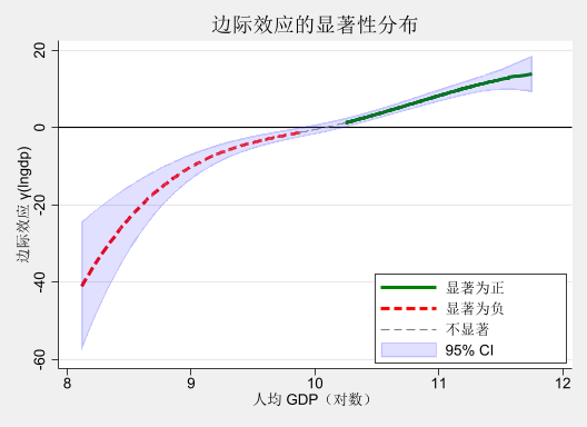
lngdp < 9 :边际效应为负 → 经济欠发达地区,ER 抑制 GTI9 < lngdp < 10 :边际效应接近 0 → 过渡阶段lngdp > 10 :边际效应为正且增强 → 经济发达地区,ER 促进 GTI
gen significant = 0replace significant = 1 if fcoe_lb > 0 // 显著为正 replace significant = -1 if fcoe_ub < 0 // 显著为负 label define sig_lab -1 "显著为负" 0 "不显著" 1 "显著为正" label values significant sig_lab
(630 real changes made)
(557 real changes made)
twoway (line fcoe_gti_1 lngdp if significant==1, lcolor(green ) lwidth(thick) sort ) /// line fcoe_gti_1 lngdp if significant==-1, lcolor(red ) lwidth(thick) sort ) /// line fcoe_gti_1 lngdp if significant==0, lcolor(gray ) lpattern(dash ) sort ) /// color (blue %15) sort ), /// yline (0, lcolor(black )) /// xtitle ("人均 GDP(对数)" ) /// ytitle ("边际效应 γ(lngdp)" ) /// title ("边际效应的显著性分布" ) /// legend (order (1 "显著为正" 2 "显著为负" 3 "不显著" 4 "95% CI" ) /// ring (0) pos(5) c(1)) /// scheme (s2mono)
tab significant, missing
significant |      Freq.     Percent        Cum.
------------+-----------------------------------
   显著为负 |        557       37.89       37.89
     不显著 |        283       19.25       57.14
   显著为正 |        630       42.86      100.00
------------+-----------------------------------
      Total |      1,470      100.00